Streaming Inference with Convolutional Layers

In this post, we explore how to apply convolutional layers to infinitely long inputs, specifically focusing on how to process inputs in chunks to minimize latency. For instance, in text-to-speech applications, instead of synthesizing an entire sentence at once, we prefer to generate and play back audio in segments. While recurrent or autoregressive networks are inherently causal and thus well-suited for streaming processing, convolutional layers present more challenges and require careful handling.

Conv1d

First, let’s examine a standard convolutional layer. By default, convolutions are non-causal, meaning the output at any given time may depend on both past and future input values.

Non-causal convolution

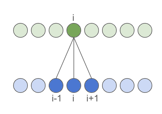
To achieve output of the same size as the input, we pad the input on both sides by the receptive_field of the convolution layer, defined as kernel_size // 2:

import torch

x = torch.randn(1, 1, 100)  # (batch x channels x time)
kernel_size = 7
receptive_field = kernel_size // 2
non_causal_conv_layer = torch.nn.Conv1d(
    1,  # input channels
    1,  # output channels
    kernel_size,
    bias=False,
    padding=receptive_field,
)

y = non_causal_conv_layer(x)
assert x.shape == y.shape

For chunked inference, padding must be applied manually, and the input shifted by chunk_size - 2 * receptive_field for each subsequent chunk.

Non-causal convolution in chunks

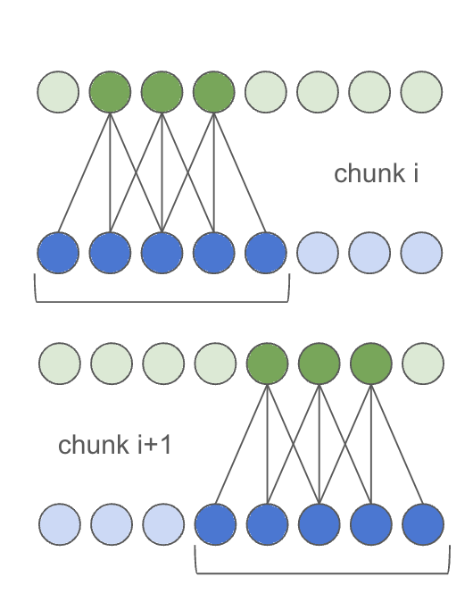
This can be implemented as follows:

non_causal_chunk_conv_layer = torch.nn.Conv1d(
    1,  # input channels
    1,  # output channels
    kernel_size,
    bias=False,
    padding=0,  # we will do padding manually
)
# copy the weights from the original conv layer
non_causal_chunk_conv_layer.weight = non_causal_conv_layer.weight
# pad the input by receptive field on both sides
padded_x = torch.nn.functional.pad(x, (receptive_field, receptive_field))

# run inference in a loop on chunk_size
chunk_outputs = []
chunk_size = 20
i = 0
while i < padded_x.size(2) - 2 * receptive_field:
    chunk = padded_x[:, :, i: i + chunk_size + 2 * receptive_field]
    chunk_outputs.append(
        non_causal_chunk_conv_layer(chunk)
    )
    i += chunk_size
chunked_y = torch.cat(chunk_outputs, 2)
assert chunked_y.shape == y.shape
assert torch.all(chunked_y == y)

If you have a stack of convolutional layers, their receptive fields simply add up, but the method remains the same.

Causal Conv1d

For online processing (such as live denoising or voice conversion), latency is influenced by both chunk_size and the receptive_field of the convolutional kernel on the right, also known as lookahead. While chunk size is adjustable, the receptive field is limited by the architecture. To reduce latency, one should aim to design a convolution with an asymmetrical receptive field. In the extreme case, with no lookahead, this results in a causal convolutional layer:

Causal convolution

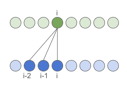
This is achieved by asymmetrically padding the convolution, padding only on the left by kernel_size - 1:

causal_conv_layer = torch.nn.Conv1d(
    1,  # input channels
    1,  # output channels
    kernel_size,
    bias=False,
    padding=0,  # need to do padding manually for assymetric case
)
padded_x = torch.nn.functional.pad(x, (kernel_size - 1, 0))

y = causal_conv_layer(padded_x)
assert x.shape == y.shape

Inference in chunks does not differ significantly from a regular convolution, except that there is only one receptive field located on the left of the input.

# run inference in a loop on chunk_size
chunk_outputs = []
chunk_size = 20
i = 0
receptive_field = kernel_size - 1
while i < padded_x.size(2) - receptive_field:
    chunk = padded_x[:, :, i: i + chunk_size + receptive_field]
    chunk_outputs.append(
        causal_conv_layer(chunk)
    )
    i += chunk_size
chunked_y = torch.cat(chunk_outputs, 2)
assert chunked_y.shape == y.shape
assert torch.all(chunked_y == y)

Transposed Conv1d

In audio or image processing, low-dimensional latent representations often need to be upsampled back to samples or pixels. This is achieved through transposed convolution with strides. A detailed explanation of this can be found in a blogpost on the topic. In short, each input point expands into multiple output points. The stride determines the degree of upsampling performed by the transposed convolution, usually set so kernel_size = stride * 2 to prevent checkboard artifacts. Two neighboring input points contribute to each output point. Padding in this case actually reduces the number of output points at the edges, ensuring that stride * len(input) output points are produced.

Transposed convolution with stride

import torch

upsample_rate = 4
kernel_size = upsample_rate * 2 + upsample_rate % 2
padding = (kernel_size - upsample_rate) // 2

transposed_conv_layer = torch.nn.ConvTranspose1d(
    in_channels=1,
    out_channels=1,
    kernel_size=kernel_size,
    stride=upsample_rate,
    padding=padding,
    bias=False,
)

y = transposed_conv_layer(x)  # (1, 1, 400)
print(y.shape)
assert y.shape == (x.size(0), x.size(1), x.size(2) * upsample_rate)

Running transposed convolution in chunks is similar to regular convolution: edges of the output are trimmed, input is padded, and inference is performed on overlapping chunks.

Transposed convolution with stride in chunks

Computing parameters for streaming inference differs from regular convolution:

# we will run inference with overlap,
# which needs to be taken into account
# in the slicing
extra_samples = (kernel_size - upsample_rate) * 3 // 2 - upsample_rate % 2  # how much extra output samples on the left and right
transposed_chunk_conv_layer = torch.nn.ConvTranspose1d(
    in_channels=1,
    out_channels=1,
    kernel_size=kernel_size,
    stride=upsample_rate,
    padding=extra_samples,
    bias=False
)
transposed_chunk_conv_layer.weight = transposed_conv_layer.weight

chunk_outputs = []
chunk_size = 20
i = 0
# each output contributed by 2 inputs, so overlap is 1
overlap = kernel_size // (2 * upsample_rate)
# need to pad so edges are handled correctly,
# this padding is taken into account in slicing
padded_x = torch.nn.functional.pad(x, (overlap, overlap))
while i < padded_x.size(2) - 2 * overlap:
    chunk = padded_x[:, :, i: i + chunk_size + 2 * overlap]
    res = transposed_chunk_conv_layer(chunk)
    chunk_outputs.append(res)
    i += chunk_size
chunked_y = torch.cat(chunk_outputs, 2)
assert chunked_y.shape == y.shape
assert torch.all(chunked_y == y)

Fourier transform

Many image and audio processing techniques still incorporate elements from classical signal processing. For audio, it’s common to extract a spectrogram to downsample the redundant audio signal while preserving the most relevant information. During training, this can be achieved using torch.stft. When deploying the model, however, there are challenges in tracing this operation across different CPU and GPU precisions. A workaround involves reformulating spectrogram extraction as a convolution with strides. This approach is already implemented in nnAudio. Here, the STFT is executed with a precomputed convolution where the kernel size matches the number of FFT points and the stride equals the hop size between windows.

Extracting spectrogram looks like this:

import torch
from nnAudio.features.stft import STFT

win_length = 1024
downsample_rate = 320
stft = STFT(
    n_fft=win_length,
    win_length=win_length,
    hop_length=downsample_rate,
    # disabling padding
    # https://github.com/KinWaiCheuk/nnAudio/blob/9e9a4bad230d175f7ad541309829483f1274a3e5/Installation/nnAudio/features/stft.py#L278
    center=False,
    output_format="Magnitude",
    pad_mode="constant"
)

total_frames = 30
total_samples = win_length + (total_frames - 1) * downsample_rate
x = torch.randn(1, total_samples)
y = stft(x)
assert y.size(2) == total_frames

When computing the spectrogram in chunks, the same approach is applied as with causal convolution:

chunk_size = 5
chunk_size_samples = chunk_size * downsample_rate
# overlap between the frames
receptive = win_length - downsample_rate
start = 0
chunked_y_lst = []
while start <= x.size(1) - chunk_size_samples - receptive:
    chunk = x[:, start:start + chunk_size_samples + receptive]
    chunked_y_lst.append(stft(chunk))
    start += chunk_size_samples
chunked_y = torch.cat(chunked_y_lst, dim=2)
assert chunked_y.shape == y.shape
assert torch.all(torch.abs(chunked_y - y) < 1e-3)

Putting it all together

Let’s integrate everything and examine how layers might interact in a typical audio-to-audio stack, where audio is first downsampled to a latent representation and then upsampled back. The model might look something like this:

from typing import List
import torch
from nnAudio.features.stft import STFT

def create_conv_stack(kernels: List[int], in_channels: int = 1) -> torch.nn.Sequential:
    """
    Creates a dummy convolutional stack
    """
    lst = []
    for i, k in enumerate(kernels):
        ic = in_channels if i == 0 else 1
        lst.append(
            torch.nn.Conv1d(
                ic,  # input channels
                1,  # output channels
                k,
                bias=False,
                padding=0,
            )
        )
    return torch.nn.Sequential(*lst)

def create_transpose_conv(upsample_rate: int) -> torch.nn.ConvTranspose1d:
    """
    Creates dummy transposed convolutional layer that upsamples the input signal
    by given ratio
    """
    kernel_size = upsample_rate * 2 + upsample_rate % 2
    extra_samples = (kernel_size - upsample_rate) * 3 // 2 - upsample_rate % 2
    return torch.nn.ConvTranspose1d(
        in_channels=1,
        out_channels=1,
        kernel_size=kernel_size,
        stride=upsample_rate,
        padding=extra_samples,
        bias=False
    )

"""
Finally the model, which is a stack of
STFT -> conv_stack -> in_conv -> upsampling -> conv_stack -> upsampling -> conv_stack -> out_conv
"""
model = torch.nn.Sequential(
    STFT(
        n_fft=1024,
        win_length=1024,
        hop_length=320,
        center=False,  # disables the padding
        output_format="Magnitude",
        pad_mode="constant"
    ),
    create_conv_stack([5, 5, 5], 513),
    create_conv_stack([7]),
    create_transpose_conv(5),
    create_conv_stack([3, 5, 11]),
    create_transpose_conv(64),
    create_conv_stack([3, 5, 11]),
    create_conv_stack([7]),
)

Given what we’ve learnt so far, lets define the receptive field for each layer, to understand how much context on the left and on the right our model requires

# define receptive fields of each layer in the stack
# for each layer, specify (left_receptive, right_receptive, resolution)
# notice how STFT and transposed conv layers change the resolution
receptives_with_resolutions = [
    (1024 - 320, 0, 1),  # STFT: requires (win_len - hop_size) on the left 
    ((5 - 1) * 3, 0, 320),  # conv_stack: 3 causal layers with receptive of (kernel_size - 1) 
    (7 // 2, 7 // 2, 320), # in_conv: non-causal conv layer with symmetric repective of kernel_size // 2
    (1, 1, 320),  # transposed conv: receptive is defined by overlap = kernel_size // (2 * upsample_rate) == 1
    (2 + 4 + 10, 0, 64),  # conv_stack: 3 causal layers with varying kernel_size
    (1, 1, 64),  # transposed conv: different upsample rate, but it doesn't affect overlap
    (2 + 4 + 10, 0, 1),  # conv_stack: another 3 causal layers with varying kernel_size
    (7 // 2, 7 // 2, 1), # out_conv: another non-causal conv layer with symmetric repective
]
# bring all to the same resolution (samples)
receptives = [(left * res, right * res) for left, right, res in receptives_with_resolutions]
# this is our overlap in case of chunked synthesis
left = sum([left for left, _ in receptives])  # 6931
# and this is our architectural latency, in case of online processing
right = sum([right for _, right in receptives])  # 1347

To confirm that we calculated the receptive field correctly, we can run the model on a dummy input and check the input/output dimensionality. The input length should be compatible with model downsampling. In our case, the input length should generate a whole number of outputs for the STFT layer. This is the case if input_length = hop_length * N + win_length.

input_length = 320 * 50 + 1024
x = torch.zeros(1, input_length)
y = model(x)
# if we calculated receptive field correctly,
# model should strip off left/right receptives
assert input_length - left - right == y.size(2)

From previous examples, for inference in chunks, we need to shift the input by chunk_size, which is the input size without receptive fields. In our case, the chunk_size is 320 * N + 1024 - left - right. For N==50, it is 8746. There is a problem, however. We can only shift the input by the stride of the downsampling layer(s), in our case by M * 320. For most architectures, there is no way to satisfy both requirements:

• Shift by chunk_size
• Shift by M * downsampling_stride To overcome this issue, we’ll have to drop some extra samples from the output, in order to be able to do inference in chunks:

chunk_size = input_length - left - right  # 8746
extra_to_drop = chunk_size % 320  # 106

Now we are all set to check if inference in chunks works. As before, for a dummy input we will run inference on the whole input, and then on chunks of the input and compare the results.

# some random input
x = torch.randn((1, 100000))
# inference on the whole input
y = model(x)

# running inference on the first chunk
y_chunk_1 = model(x[:, :input_length])
# running inference on the second chunk, carefully shifting input
start = chunk_size - extra_to_drop
y_chunk_2 = model(x[:, start:(start + input_length)])
# now we need to slice off the `extra_to_drop` from both outputs
y_chunk_list = [y_chunk_1, y_chunk_2]
y_chunk_list = [chunk[:, :, :-extra_to_drop] for chunk in y_chunk_list]
y_chunk = torch.cat(y_chunk_list, dim=2)

# finally compare the chunked inference to the original one.
# we run inference only on two chunks, omitting handling the
# padding on the right for simplicity. So the comparison
# is done only for beginning of the output.
diff = y[:, :, :y_chunk.size(2)] - y_chunk
# should be the same
assert torch.all(torch.abs(diff) < 1e-3)

Takeaways

In this post, we delved into how to perform streaming inference (a.k.a., inference in chunks) for models consisting of various convolutional layers. This insight is crucial for building online audio or image processing applications. It boils down to carefully computing the receptive field of the resulting model and managing overlap between input chunks. When multiple layers are combined, however, additional attention should be paid to feeding your model with input of proper length, which in turn requires more sophisticated input/output handling. Hopefully, the explanations and code snippets provided will help you navigate these challenges in your own architectural designs.