While ELO-based ranking relies on human judgment, objective metrics are also commonly used for leaderboards. Though speech generation lacks a universal standard for objective evaluation, the community has developed several useful metrics:

• Intelligibility - measured by speech recognition error rates on synthetic speech
• Naturalness - predicted using models trained on human naturalness ratings
• Similarity - for voice cloning systems, measured by cosine similarity between speaker embeddings of reference and generated speech

We would like to introduce:

speech_gen_eval (github)

An open-source library for objective evaluation of speech generation models

speech_gen_eval_testsets (huggingface)

A collection of test sets for evaluating speech generation models

speech_gen_baselines (huggingface)

A dataset containing synthetic speech from common models and their evaluation results

TTSLeaderboard (huggingface)

A leaderboard for speech generation models

There are other tools for objective evaluation of speech generation, including ZS-TTS-Evaluation, seed-tts-eval, tts-scores, evaluate-zero-shot-tts, and another leaderboard called TTSDS Scores. Our contribution focuses on:

• Simple addition of new metrics and test sets
• Support for various speech generation models (vocoders, zero-shot TTS, zero-shot VC, etc.), where tools can be reused
• Mature engineering with easy installation and fast evaluation
• Allowing to listen to the generated speech side-by-side to build a relation between metrics and perceived quality

Having most of these tools internally for a while, we are now making them publicly available.

We plan to expand the leaderboard with more models and add new metrics to the library. We welcome your suggestions and contributions!

Tracing

Converting model into Torch JIT file allows to run inference with minimal dependencies (just PyTorch) or deployment on inference servers (e.g. Triton). In this tracing, we integrate the clustering step into the Torch module, eliminating the need to carry around custom clustering code.

Unfortunately, the FAISS index for clustering step is only available for model after the second iteration. As a result, the traced model is slightly less capable.

The traced model is available at balacoon/mhubert-147. The full notebook used for tracing and testing can be found here.

Many thanks to @dathudeptrai for posting a snippet on discrete tokens extraction.

Notes

Here are some notes and practical findings from the mHuBERT model tracing. Please drop a message if any of these are incorrect or incomplete.

• The attention mask is ignored by mHuBERT. As a result, during batched inference, you can get different discrete codes depending on the padding:

• mHuBERT applies mean/std normalization to input audio.
• faiss has a lot of clustering methods implemented. Fortunately a linear transformation was used for clustering in mHuBERT, allowing it to be extracted into a transformation matrix. See TorchFaiss in the notebook for details.

Methods

We compare the following methods:

• SoX - vanilla upsampling via interpolation, the higher frequencies are not restored.
• Resemble Enhance - diffusion-based denoising / enhancement / upsampling.
• AudioSR - diffusion-based audio super resolution.
• AP-BWE - GAN-based bandwidth extension in spectral domain.

Processing speed per file on a single RTX 3090:

We measure intelligibility, audio quality and speaker similarity of the processed audio on two datasets: VCTK[2] and DAPS[3]. First represents clean audio that simply lacks higher frequencies. Second - is a more challenging usecase of speech recorded on consumer microphones with background noise present. We use ECAPA[4] speaker encoder by Speechbrain to extract speaker representation and measure speaker similarity. We run speech recognition with Conformer-Transducer ASR model by NVIDIA to evaluate intelligibility in terms of Character Error Rate. Finally, we use a pre-trained Mean Opinion Score estimator UTMOS[5] to access the naturalness. Keep in mind that all the metrics are computed on 16khz audio, so they are mainly tracking if upsampling introduces any changes to the information that is already there.

VCTK testset

A 2k subset is sampled.

Example of the upsampling in spectral domain:

Audio samples:

DAPS testset

Dataset is segmented into sentence-level, a 2k subset is sampled.

Example of the upsampling in spectral domain:

Audio samples:

Conclusions

Resemble-Enhance strives to also perform denoising and enhancement. It corrupts the noisy audio files substantially which is reflected in greatly degraded intelligibility. Both AudioSR and AP-BWE are very gentle to existing information and do not change the metrics. Former adds more details and combines with existing high-freq information more smoothly. Latter is however almost 150x faster. Our pick is AudioSR if the amount of data is managable, otherwise AP-BWE.

References

[1] LibriTTS-R: A Restored Multi-Speaker Text-to-Speech Corpus

[2] CSTR VCTK Corpus: English Multi-speaker Corpus for CSTR Voice Cloning Toolkit

[3] Device and Produced Speech (DAPS) Dataset

[4] ECAPA-TDNN Embeddings for Speaker Diarization

[5] UTMOS: UTokyo-SaruLab System for VoiceMOS Challenge 2022

Conv1d

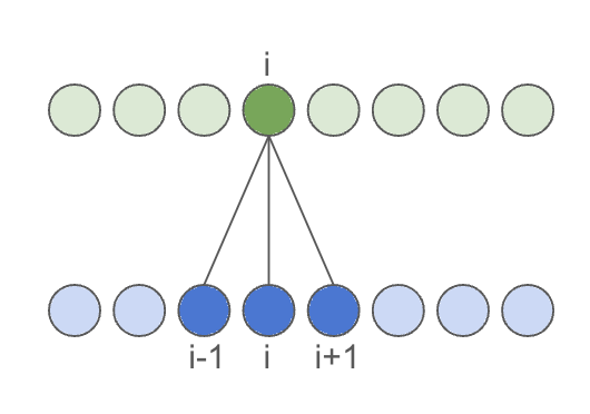
First, let’s examine a standard convolutional layer. By default, convolutions are non-causal, meaning the output at any given time may depend on both past and future input values.

To achieve output of the same size as the input, we pad the input on both sides by the receptive_field of the convolution layer, defined as kernel_size // 2:

import torch

x = torch.randn(1, 1, 100)  # (batch x channels x time)
kernel_size = 7
receptive_field = kernel_size // 2
non_causal_conv_layer = torch.nn.Conv1d(
    1,  # input channels
    1,  # output channels
    kernel_size,
    bias=False,
    padding=receptive_field,
)

y = non_causal_conv_layer(x)
assert x.shape == y.shape

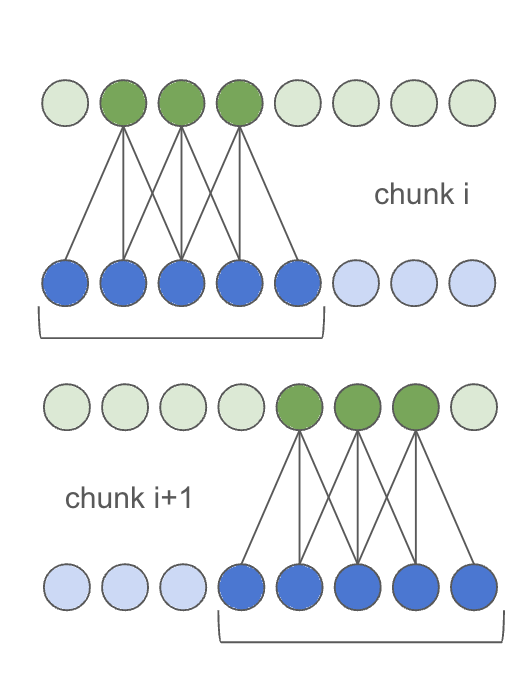
For chunked inference, padding must be applied manually, and the input shifted by chunk_size - 2 * receptive_field for each subsequent chunk.

This can be implemented as follows:

non_causal_chunk_conv_layer = torch.nn.Conv1d(
    1,  # input channels
    1,  # output channels
    kernel_size,
    bias=False,
    padding=0,  # we will do padding manually
)
# copy the weights from the original conv layer
non_causal_chunk_conv_layer.weight = non_causal_conv_layer.weight
# pad the input by receptive field on both sides
padded_x = torch.nn.functional.pad(x, (receptive_field, receptive_field))

# run inference in a loop on chunk_size
chunk_outputs = []
chunk_size = 20
i = 0
while i < padded_x.size(2) - 2 * receptive_field:
    chunk = padded_x[:, :, i: i + chunk_size + 2 * receptive_field]
    chunk_outputs.append(
        non_causal_chunk_conv_layer(chunk)
    )
    i += chunk_size
chunked_y = torch.cat(chunk_outputs, 2)
assert chunked_y.shape == y.shape
assert torch.all(chunked_y == y)

If you have a stack of convolutional layers, their receptive fields simply add up, but the method remains the same.

Causal Conv1d

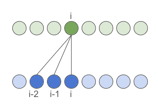
For online processing (such as live denoising or voice conversion), latency is influenced by both chunk_size and the receptive_field of the convolutional kernel on the right, also known as lookahead. While chunk size is adjustable, the receptive field is limited by the architecture. To reduce latency, one should aim to design a convolution with an asymmetrical receptive field. In the extreme case, with no lookahead, this results in a causal convolutional layer:

This is achieved by asymmetrically padding the convolution, padding only on the left by kernel_size - 1:

causal_conv_layer = torch.nn.Conv1d(
    1,  # input channels
    1,  # output channels
    kernel_size,
    bias=False,
    padding=0,  # need to do padding manually for assymetric case
)
padded_x = torch.nn.functional.pad(x, (kernel_size - 1, 0))

y = causal_conv_layer(padded_x)
assert x.shape == y.shape

Inference in chunks does not differ significantly from a regular convolution, except that there is only one receptive field located on the left of the input.

# run inference in a loop on chunk_size
chunk_outputs = []
chunk_size = 20
i = 0
receptive_field = kernel_size - 1
while i < padded_x.size(2) - receptive_field:
    chunk = padded_x[:, :, i: i + chunk_size + receptive_field]
    chunk_outputs.append(
        causal_conv_layer(chunk)
    )
    i += chunk_size
chunked_y = torch.cat(chunk_outputs, 2)
assert chunked_y.shape == y.shape
assert torch.all(chunked_y == y)

Transposed Conv1d

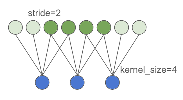
In audio or image processing, low-dimensional latent representations often need to be upsampled back to samples or pixels. This is achieved through transposed convolution with strides. A detailed explanation of this can be found in a blogpost on the topic. In short, each input point expands into multiple output points. The stride determines the degree of upsampling performed by the transposed convolution, usually set so kernel_size = stride * 2 to prevent checkboard artifacts. Two neighboring input points contribute to each output point. Padding in this case actually reduces the number of output points at the edges, ensuring that stride * len(input) output points are produced.

import torch

upsample_rate = 4
kernel_size = upsample_rate * 2 + upsample_rate % 2
padding = (kernel_size - upsample_rate) // 2

transposed_conv_layer = torch.nn.ConvTranspose1d(
    in_channels=1,
    out_channels=1,
    kernel_size=kernel_size,
    stride=upsample_rate,
    padding=padding,
    bias=False,
)

y = transposed_conv_layer(x)  # (1, 1, 400)
print(y.shape)
assert y.shape == (x.size(0), x.size(1), x.size(2) * upsample_rate)

Running transposed convolution in chunks is similar to regular convolution: edges of the output are trimmed, input is padded, and inference is performed on overlapping chunks.

Computing parameters for streaming inference differs from regular convolution:

# we will run inference with overlap,
# which needs to be taken into account
# in the slicing
extra_samples = (kernel_size - upsample_rate) * 3 // 2 - upsample_rate % 2  # how much extra output samples on the left and right
transposed_chunk_conv_layer = torch.nn.ConvTranspose1d(
    in_channels=1,
    out_channels=1,
    kernel_size=kernel_size,
    stride=upsample_rate,
    padding=extra_samples,
    bias=False
)
transposed_chunk_conv_layer.weight = transposed_conv_layer.weight

chunk_outputs = []
chunk_size = 20
i = 0
# each output contributed by 2 inputs, so overlap is 1
overlap = kernel_size // (2 * upsample_rate)
# need to pad so edges are handled correctly,
# this padding is taken into account in slicing
padded_x = torch.nn.functional.pad(x, (overlap, overlap))
while i < padded_x.size(2) - 2 * overlap:
    chunk = padded_x[:, :, i: i + chunk_size + 2 * overlap]
    res = transposed_chunk_conv_layer(chunk)
    chunk_outputs.append(res)
    i += chunk_size
chunked_y = torch.cat(chunk_outputs, 2)
assert chunked_y.shape == y.shape
assert torch.all(chunked_y == y)

Fourier transform

Many image and audio processing techniques still incorporate elements from classical signal processing. For audio, it’s common to extract a spectrogram to downsample the redundant audio signal while preserving the most relevant information. During training, this can be achieved using torch.stft. When deploying the model, however, there are challenges in tracing this operation across different CPU and GPU precisions. A workaround involves reformulating spectrogram extraction as a convolution with strides. This approach is already implemented in nnAudio. Here, the STFT is executed with a precomputed convolution where the kernel size matches the number of FFT points and the stride equals the hop size between windows.

Extracting spectrogram looks like this:

import torch
from nnAudio.features.stft import STFT

win_length = 1024
downsample_rate = 320
stft = STFT(
    n_fft=win_length,
    win_length=win_length,
    hop_length=downsample_rate,
    # disabling padding
    # https://github.com/KinWaiCheuk/nnAudio/blob/9e9a4bad230d175f7ad541309829483f1274a3e5/Installation/nnAudio/features/stft.py#L278
    center=False,
    output_format="Magnitude",
    pad_mode="constant"
)

total_frames = 30
total_samples = win_length + (total_frames - 1) * downsample_rate
x = torch.randn(1, total_samples)
y = stft(x)
assert y.size(2) == total_frames

When computing the spectrogram in chunks, the same approach is applied as with causal convolution:

chunk_size = 5
chunk_size_samples = chunk_size * downsample_rate
# overlap between the frames
receptive = win_length - downsample_rate
start = 0
chunked_y_lst = []
while start <= x.size(1) - chunk_size_samples - receptive:
    chunk = x[:, start:start + chunk_size_samples + receptive]
    chunked_y_lst.append(stft(chunk))
    start += chunk_size_samples
chunked_y = torch.cat(chunked_y_lst, dim=2)
assert chunked_y.shape == y.shape
assert torch.all(torch.abs(chunked_y - y) < 1e-3)

Inverse Fourier transform

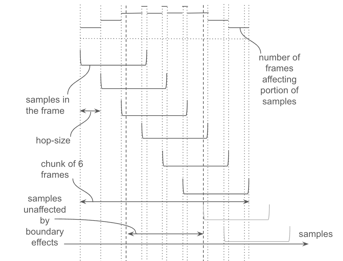
The inverse Fourier transform is surprisingly more complex. Let’s revisit the audio example to understand why. Overlapping frames create interesting patterns that influence which frames affect which samples in the output.

In the illustration above, a chunk of 6 frames is shown with framing parameters of n_fft = 1024 and hop_length = 320. Since n_fft % hop_length != 0, the number of frames that affect the output samples varies between 3 and 4. For the edges of the input, it is fewer, and these regions should be considered the receptive field.

Just like before, executing the inverse Short-Time Fourier Transform (iSTFT) on the entire input:

import torch
from nnAudio.features.stft import iSTFT

win_length = 1024
upsample_rate = 320
istft = iSTFT(
    n_fft=win_length,
    win_length=win_length,
    hop_length=upsample_rate,
    center=False,
)

total_frames = 100
x = torch.randn(1, win_length//2 + 1, total_frames, 2)
y = istft(x, onesided=True)

receptive = win_length - upsample_rate
# to have an even upsampling, we should slice half of the receptive.
# this leaves some edge effects however 
y_padded = y[:, receptive // 2:-receptive // 2]
assert y_padded.size(1) == total_frames * upsample_rate
# keeping only output that doesn't have edge effects,
# we need to slice off entire receptive field
y = y[:, receptive:-receptive]

Running in chunks includes manual slicing from the output of the iSTFT, to remove regions without boundary effects:

import numpy as np

chunked_y_lst = []
start = 0
chunk_size = 5
overlap = int(win_length / upsample_rate)
while start <= total_frames - chunk_size:
    chunk = x[:, :, start:start + chunk_size + overlap]
    chunk_out = istft(chunk, onesided=True)
    left = win_length - win_length % upsample_rate
    right = receptive
    chunk_out = chunk_out[:, left:-right]

    chunked_y_lst.append(chunk_out)
    start += chunk_size

chunked_y = torch.cat(chunked_y_lst, dim=1)
# some of the original output is lost
lost = upsample_rate - win_length % upsample_rate
y_with_lost = y[:, lost:chunked_y.size(1) + lost]

assert torch.mean(torch.abs(chunked_y - y_with_lost)) < 1e-5

Putting it all together (Transposed Conv)

Let’s integrate everything and examine how layers might interact in a typical audio-to-audio stack, where audio is first downsampled to a latent representation and then upsampled back. The model might look something like this:

from typing import List
import torch
from nnAudio.features.stft import STFT

def create_conv_stack(kernels: List[int], in_channels: int = 1) -> torch.nn.Sequential:
    """
    Creates a dummy convolutional stack
    """
    lst = []
    for i, k in enumerate(kernels):
        ic = in_channels if i == 0 else 1
        lst.append(
            torch.nn.Conv1d(
                ic,  # input channels
                1,  # output channels
                k,
                bias=False,
                padding=0,
            )
        )
    return torch.nn.Sequential(*lst)

def create_transpose_conv(upsample_rate: int) -> torch.nn.ConvTranspose1d:
    """
    Creates dummy transposed convolutional layer that upsamples the input signal
    by given ratio
    """
    kernel_size = upsample_rate * 2 + upsample_rate % 2
    extra_samples = (kernel_size - upsample_rate) * 3 // 2 - upsample_rate % 2
    return torch.nn.ConvTranspose1d(
        in_channels=1,
        out_channels=1,
        kernel_size=kernel_size,
        stride=upsample_rate,
        padding=extra_samples,
        bias=False
    )

"""
Finally the model, which is a stack of
STFT -> conv_stack -> in_conv -> upsampling -> conv_stack -> upsampling -> conv_stack -> out_conv
"""
model = torch.nn.Sequential(
    STFT(
        n_fft=1024,
        win_length=1024,
        hop_length=320,
        center=False,  # disables the padding
        output_format="Magnitude",
        pad_mode="constant"
    ),
    create_conv_stack([5, 5, 5], 513),
    create_conv_stack([7]),
    create_transpose_conv(5),
    create_conv_stack([3, 5, 11]),
    create_transpose_conv(64),
    create_conv_stack([3, 5, 11]),
    create_conv_stack([7]),
)

Given what we’ve learnt so far, lets define the receptive field for each layer, to understand how much context on the left and on the right our model requires

# define receptive fields of each layer in the stack
# for each layer, specify (left_receptive, right_receptive, resolution)
# notice how STFT and transposed conv layers change the resolution
receptives_with_resolutions = [
    (1024 - 320, 0, 1),  # STFT: requires (win_len - hop_size) on the left 
    ((5 - 1) * 3, 0, 320),  # conv_stack: 3 causal layers with receptive of (kernel_size - 1) 
    (7 // 2, 7 // 2, 320), # in_conv: non-causal conv layer with symmetric repective of kernel_size // 2
    (1, 1, 320),  # transposed conv: receptive is defined by overlap = kernel_size // (2 * upsample_rate) == 1
    (2 + 4 + 10, 0, 64),  # conv_stack: 3 causal layers with varying kernel_size
    (1, 1, 64),  # transposed conv: different upsample rate, but it doesn't affect overlap
    (2 + 4 + 10, 0, 1),  # conv_stack: another 3 causal layers with varying kernel_size
    (7 // 2, 7 // 2, 1), # out_conv: another non-causal conv layer with symmetric repective
]
# bring all to the same resolution (samples)
receptives = [(left * res, right * res) for left, right, res in receptives_with_resolutions]
# this is our overlap in case of chunked synthesis
left = sum([left for left, _ in receptives])  # 6931
# and this is our architectural latency, in case of online processing
right = sum([right for _, right in receptives])  # 1347

To confirm that we calculated the receptive field correctly, we can run the model on a dummy input and check the input/output dimensionality. The input length should be compatible with model downsampling. In our case, the input length should generate a whole number of outputs for the STFT layer. This is the case if input_length = hop_length * N + win_length.

input_length = 320 * 50 + 1024
x = torch.zeros(1, input_length)
y = model(x)
# if we calculated receptive field correctly,
# model should strip off left/right receptives
assert input_length - left - right == y.size(2)

From previous examples, for inference in chunks, we need to shift the input by chunk_size, which is the input size without receptive fields. In our case, the chunk_size is 320 * N + 1024 - left - right. For N==50, it is 8746. There is a problem, however. We can only shift the input by the stride of the downsampling layer(s), in our case by M * 320. For most architectures, there is no way to satisfy both requirements:

• Shift by chunk_size
• Shift by M * downsampling_stride To overcome this issue, we’ll have to drop some extra samples from the output, in order to be able to do inference in chunks:

chunk_size = input_length - left - right  # 8746
extra_to_drop = chunk_size % 320  # 106

Now we are all set to check if inference in chunks works. As before, for a dummy input we will run inference on the whole input, and then on chunks of the input and compare the results.

# some random input
x = torch.randn((1, 100000))
# inference on the whole input
y = model(x)

# running inference on the first chunk
y_chunk_1 = model(x[:, :input_length])
# running inference on the second chunk, carefully shifting input
start = chunk_size - extra_to_drop
y_chunk_2 = model(x[:, start:(start + input_length)])
# now we need to slice off the `extra_to_drop` from both outputs
y_chunk_list = [y_chunk_1, y_chunk_2]
y_chunk_list = [chunk[:, :-extra_to_drop] for chunk in y_chunk_list]
y_chunk = torch.cat(y_chunk_list, dim=2)

# finally compare the chunked inference to the original one.
# we run inference only on two chunks, omitting handling the
# padding on the right for simplicity. So the comparison
# is done only for beginning of the output.
diff = y[:, :, :y_chunk.size(2)] - y_chunk
# should be the same
assert torch.all(torch.abs(diff) < 1e-3)

Putting it all together (iSTFT)

Now, let’s do the same, but replace the upsampling with transposed convolutions and use the inverse STFT (iSTFT). Once again, we will ensure that carefully computing the total receptive field of all layers allows us to run inference on chunks of input.

Model definition:

from typing import List
import torch
from nnAudio.features.stft import STFT, iSTFT

def create_conv_stack(kernels: List[int], in_channels: int, out_channels: int) -> torch.nn.Sequential:
    """
    Creates a dummy convolutional stack
    """
    lst = []
    for i, k in enumerate(kernels):
        ic = in_channels if i == 0 else out_channels
        lst.append(
            torch.nn.Conv1d(
                ic,  # input channels
                out_channels,  # output channels
                k,
                bias=False,
                padding=0,
            )
        )
    return torch.nn.Sequential(*lst)

class iSTFTWrap(torch.nn.Module):
    def __init__(self, n_fft, hop_length):
        super().__init__()
        self._istft = iSTFT(
            n_fft=n_fft,
            win_length=n_fft,
            hop_length=hop_length,
            center=False,
        )
        self._left = n_fft - n_fft % hop_length
        self._right = n_fft - hop_length
    
    def forward(self, x: torch.Tensor) -> torch.Tensor:
        # the input x is (batch x 1026 x frames)
        x = x.view(x.size(0), 2, x.size(1) // 2, x.size(2))  # (batch x 2 x 513 x frames)
        x = x.permute(0, 2, 3, 1)  # (batch x 513 x frames x 2)
        y = self._istft(x, onesided=True)
        return y[:, self._left:-self._right]

"""
Finally the model, which is a stack of
STFT -> conv_stack -> out_conv -> iSTFT
"""
model = torch.nn.Sequential(
    STFT(
        n_fft=1024,
        win_length=1024,
        hop_length=320,
        center=False,  # disables the padding
        output_format="Magnitude",
        pad_mode="constant"
    ),
    create_conv_stack([5, 5, 5], 513, 1),
    create_conv_stack([7], 1, 513 * 2),
    iSTFTWrap(
        n_fft=1024,
        hop_length=320,
    )
)

# define receptive fields of each layer in the stack
# for each layer, specify (left_receptive, right_receptive, resolution)
receptives_with_resolutions = [
    (1024 - 320, 0, 1),  # STFT: requires (win_len - hop_size) on the left 
    ((5 - 1) * 3, 0, 320),  # conv_stack: 3 causal layers with receptive of (kernel_size - 1) 
    (7 // 2, 7 // 2, 320), # projection conv: non-causal conv layer with symmetric repective of kernel_size // 2
    (960, 0, 1), # iSTFT: requires hop_length * overlap * 2 on the left and receptive on the right
]
# bring all to the same resolution (samples)
receptives = [(left * res, right * res) for left, right, res in receptives_with_resolutions]
# this is our overlap in case of chunked synthesis
left = sum([left for left, _ in receptives])  # 6464
# and this is our architectural latency, in case of online processing
right = sum([right for _, right in receptives])  # 960

Now, let’s compute the expected input/output lengths. Notice that there is no extra_to_drop because the chunk size is divisible by the hop_size.

input_length = 320 * 50 + 1024
chunk_size = input_length - left - right  # 9600

Finally, let’s confirm that running inference on chunks produces the same result as when processing the entire input.

# some random input
x = torch.randn((1, 100000))
# inference on the whole input
y = model(x)

# running inference on the first chunk
y_chunk_1 = model(x[:, :input_length])
# running inference on the second chunk, carefully shifting input
start = chunk_size - extra_to_drop
y_chunk_2 = model(x[:, start:(start + input_length)])
# now we need to slice off the `extra_to_drop` from both outputs
y_chunk_list = [y_chunk_1, y_chunk_2]
if extra_to_drop > 0:
    y_chunk_list = [chunk[:, :-extra_to_drop] for chunk in y_chunk_list]
y_chunk = torch.cat(y_chunk_list, dim=1)

y_trimmed = y[:, :y_chunk.size(1)]
# finally compare the chunked inference to the original one.
# we run inference only on two chunks, omitting handling the
# padding on the right for simplicity. So the comparison
# is done only for beginning of the output.
diff = y_trimmed - y_chunk
# should be the same
assert torch.mean(torch.abs(diff)) < 1e-5

Takeaways

In this post, we delved into how to perform streaming inference (a.k.a., inference in chunks) for models consisting of various convolutional layers. This insight is crucial for building online audio or image processing applications. It boils down to carefully computing the receptive field of the resulting model and managing overlap between input chunks. When multiple layers are combined, however, additional attention should be paid to feeding your model with input of proper length, which in turn requires more sophisticated input/output handling. Hopefully, the explanations and code snippets provided will help you navigate these challenges in your own architectural designs.

• expressive speech synthesis
• paralinguistic generation
• voice cloning

These improvements became possible due to more powerful generative models and an unprecedented training scale. Instead of traditional 20 hours of speech and 10-50M parameters models, TorToiSe used thousands of hours and hundreds of millions of trainable parameters. It sparked a whole series of papers that developed the approach further, with AudioLM[2], VALL-E[3], and SPEAR-TTS[4] being the most prominent among others. In this post, we will explore the internals of the BARK - an open-source implementation of this new speech synthesis paradigm.

Architecture

BARK quite closely follows VALL-E architecture, utilizing a large autoregressive transformer decoder to operate on discrete speech representations.

Tokenization

Discrete speech representations or tokens are obtained from two pre-trained models - HuBERT[5] and Encodec[6]:

HuBERT is a semi-supervised model that converts audio to discrete “semantic tokens.” The objective of the HuBERT training makes extracted representations speaker- and prosody-(quasi)independent. Think of pseudo-phonemes annotation on a frame level.

Encodec is a neural vocoder that works on multi-level discrete representations extracted from audio in an auto-encoding manner using vector quantization. Think of mel-spectrogram frames but discrete. Low-order representations are called “coarse tokens,” and higher-order ones are “fine tokens.”

Acoustic Modeling

By discretizing the speech into tokens, we reformulate the speech production task into predicting coarse and fine tokens from semantic tokens. Such formulation allows us to use a state-of-art generative model - an autoregressive transformer decoder. The very same model is used in ChatGPT. A lot of data is needed to train this beast: billions of tokens or thousands of hours of speech. This magnitude is only possible in a multi-speaker scenario, which requires to condition a generative model on speaker identity. It is done via “prompting” (natural language processing parallels intensify), where prompt - is an utterance of a speaker predecessing the current one. The prompt carries information about speaker identity, recording conditions, and even some high-level prosody aspects, but not the actual content. Fine tokens just refine the acoustic information from coarse tokens and don’t need as powerful modeling. The transformer encoder (i.e. parallel architecture) is used for fine tokens prediction to speed things up.

Coarse and fine tokens have multiple levels. To plug them into the models, token sequences are simply flattened.

Neural Frontend

Semantic tokens are extracted from the audio. For a text-to-speech task, they need to be predicted from the input text. It is done with yet another autoregressive transformer decoder. This task also requires a powerful generative model since it contributes to the resulting intonation. Converting text to semantic tokens is a sequence-to-sequence task, where correspondence is defined by durations of sounds and overall speech pace.

A sufficiently sizeable neural frontend has no problems generating semantic tokens for inputs in multiple languages or consistently annotated paralinguistics (laughs, breaths, gasps, etc.).

Performance

Generating speech with BARK is not fast. Let’s have a look into which components are the most demanding. Measurements are done on GPU, averaging inference time for multiple utterances of roughly 10 seconds each.

Flattening coarse/fine tokens requires AR Transformer Decoder to work on a very long context. This makes it the slowest component of the whole pipeline by far.

Speeding things up

It’s not the first time slow autoregressive modeling has crossed out real-time speech generation. An autoregressive version of WaveNet[7] also puzzled the community back in the day with outstanding quality at the cost of extremely slow inference. But things got faster both with inference optimizations and modeling advances. The same applies in this case. For example, NaturalSpeech 2[8] proposes employing a parallel diffusion model instead of an autoregressive transformer decoder as a possible mitigation. We will have a brief look into possible inference optimizations.

RWKV

The quadratic complexity of attention fuels interest in so-called attention-free architectures. RWKV - is a parallelizable RNN with a performance of a classical transformer and linear complexity with respect to context length. Here is some code samples allowing to drag-race a dummy RWKV model and estimate expected gains. Creating a dummy model of 350M parameters (from within RWKV-v4):

from src.model import GPT, GPTConfig
import torch
model = GPT(GPTConfig(12096, 1024, model_type="RVKW", n_layer=24, n_embd=1024))
device = torch.device("cuda")
model.to(device)
torch.save(model.state_dict(), "rwkv_gpt2_medium.pth")

Run generation with a dummy model using rwkv from pip:

import time
import os
os.environ['RWKV_JIT_ON'] = '1'
os.environ["RWKV_CUDA_ON"] = '1'

from rwkv.model import RWKV

model = RWKV(model='rwkv_gpt2_medium.pth', strategy='cuda fp16')
state = None
# warm up
for i in range(100):
    _, state = model.forward([100], state)
# measure generation of 1k tokens
state = None
start = time.time()
for _ in range(1000):
    _, state = model.forward([100], state)
print(time.time() - start)

It takes ~12 seconds which is already a valuable improvement. It will become even more prominent with longer contexts and bigger models.

Faster Transformer

Faster Transformer is a library by NVIDIA which implements heavily optimized inference of Large Language Models. It runs in a dedicated docker container with custom CUDA kernels for particular models. Here is a small snippet of code to check out the performance on 350M GPT model:

# pulling container and building FT for you GPU
docker pull nvcr.io/nvidia/pytorch:22.09-py3
nvidia-docker run -ti --shm-size 5g --rm nvcr.io/nvidia/pytorch:22.09-py3 bash
git clone https://github.com/NVIDIA/FasterTransformer.git
mkdir -p FasterTransformer/build
cd FasterTransformer/build
git submodule init && git submodule update
# from https://github.com/NVIDIA/FasterTransformer/issues/90 for RTX3090
cmake -DSM=86 -DCMAKE_BUILD_TYPE=Release -DBUILD_PYT=ON ..
make -j12

# pulling 350M GPT model
pip install -r ../examples/pytorch/gpt/requirement.txt
git clone https://huggingface.co/gpt2-medium
curl -s https://packagecloud.io/install/repositories/github/git-lfs/script.deb.sh | bash
apt-get install git-lfs
cd gpt2-medium && git lfs pull && cd ..
python ../examples/pytorch/gpt/utils/huggingface_gpt_convert.py -i gpt2-medium/ \
    -o ../models/huggingface-models/c-model/gpt2-medium -i_g 1
echo "hello world" > context.txt

# run generation on a GPU for 1k tokens
time CUDA_VISIBLE_DEVICES=1 python ../examples/pytorch/gpt/multi_gpu_gpt_example.py \
    --ckpt_path ../models/huggingface-models/c-model/gpt2-medium/1-gpu/ \
    --time --inference_data_type fp16 --tensor_para_size 1 --pipeline_para_size 1 \
    --beam_width 1 --top_k 1 --top_p 0 --temperature 1.0 --return_cum_log_probs 0 \
    --output_len 1000  --vocab_file gpt2-medium/vocab.json --merges_file gpt2-medium/merges.txt  \
    --max_batch_size 1 --min_length 1000 --lib_path lib/libth_transformer.so \
    --sample_input_file context.txt

It takes only 1.5 seconds, a mind-blowing speed up compared to the original performance.

References

[1] Hierarchical Text-Conditional Image Generation with CLIP Latents

[2] AudioLM: a Language Modeling Approach to Audio Generation

[3] Neural Codec Language Models are Zero-Shot Text to Speech Synthesizers

[4] Speak, Read and Prompt: High-Fidelity Text-to-Speech with Minimal Supervision

[5] HuBERT: Self-Supervised Speech Representation Learning by Masked Prediction of Hidden Units

[6] High Fidelity Neural Audio Compression

[7] WaveNet: A Generative Model for Raw Audio

[8] NaturalSpeech 2: Latent Diffusion Models are Natural and Zero-Shot Speech and Singing Synthesizers

Testsets

Typical evaluations of Voice Conversion systems rely on objective metrics collected from running conversion on unseen multi-speaker corpora. We design the evaluation to be insightful for the Revoice use-case. We use multi-speaker corpora as a source or input audio and a library of speakers from Revoice app as a target or reference audio. Input audio is derived from:

• VCTK - classical voice conversion benchmark. Clean recordings, multiple accents.
• DAPS corpus[3] - emulated mobile device recordings in various conditions. This dataset resembles the audio quality we obtain as a Voice Conversion service more closely.

Metrics

We measure three model-based objective metrics for the converted speech:

• Speaker similarity: we measure a cosine distance between a latent speaker representation from converted speech and reference audio. We use ECAPA[4] speaker encoder by Speechbrain to extract speaker representation.
• Speech intelligibility: we run speech recognition with Conformer-Transducer ASR model by NVIDIA on the converted speech and measure the Character Error Rate with respect to the transcription.
• Naturalness: we use a pre-trained Mean Opinion Score estimator UTMOS[5] released by the authors.

Baselines

We select two widely-spread systems as the baselines. Both are trained on a large number of speakers and are capable of zero-shot speech generation.

• YourTTS[6] (from 2021) is a VITS architecture model with adjustments trained on VCTK + LibriTTS datasets. It uses an invertible normalizing flow to disentangle speaker identity from the spectrogram representation. Handy tutorial on how to run it can be found here.
• BARK (from 2022) is a large (350M parameters) decoder-only transformer that generates speech from “semantic tokens.” Those are self-supervised representations extracted with HuBERT[7] that effectively disentangle content (semantics) and speaker characteristics. Running Voice Conversion with BARK is not straightforward, because extraction of semantic tokens is not released. Suno.ai only provides prediction of semantic tokens from text. Fortunately, there is a community contributed semantic tokens extractors that are compatible with BARK. This addition allows to create own voice profiles and perform voice conversion, adjusting semantic tokens and voice profiles in this notebook.

The autoregressive transformer decoder in BARK is significantly slower than parallel conversion in YourTTS, but it has greater potential due to the model’s scalability.

Results

We present results of the evaluations in the tables below. Here is performance of the systems on VCTK:

And performance on DAPS:

Small example of how systems actually sound. For the these inputs:

The systems produce following outputs:

YourTTS shows excellent performance on VCTK but degrades significantly on more noisy inputs. BARK consistently delivers clean and intelligible audio, but the speaker similarity lags. Revoice competes with BARK in terms of naturalness and intelligibility while making a leap forward in terms of speaker similarity.

References

[1] Transfer Learning from Speaker Verification to Multispeaker Text-To-Speech Synthesis

[2] Neural Codec Language Models are Zero-Shot Text to Speech Synthesizers

[3] Can we Automatically Transform Speech Recorded on Common Consumer Devices in Real-World Environments into Professional Production Quality Speech? — A Dataset, Insights, and Challenges

[4] ECAPA-TDNN Embeddings for Speaker Diarization

[5] UTMOS: UTokyo-SaruLab System for VoiceMOS Challenge 2022

[6] YourTTS: Towards Zero-Shot Multi-Speaker TTS and Zero-Shot Voice Conversion for everyone

[7] HuBERT: Self-Supervised Speech Representation Learning by Masked Prediction of Hidden Units

* YourTTS uses VCTK in training, which might give slightly overly optimistic results.

Сгенеруйте більше прикладів в нашому онлайн демо.

Реліз

Дякуємо спільноті синтезу українського мовлення за створення, популяризацію і підтримку відкритих датасетів. На їх основі, ми побудували 2 моделі:

• JETS - стандартна мульти-спікер модель з частотою дискретизації 24kHz. Підтримує усі наявні голоси: Лада, Тетяна і Микита. Росповсюджується в двох варіантах:
  • uk_ltm_jets_cpu.addon - для синтезу на CPU за допомогою Python пакету balacoon_tts.
  • uk_ltm_jets_gpu.addon - для сервісу в Docker контейнері з використанням GPU.
• Light - полегшена модель з частотою дискретизації 16kHz для надшвидкої генерації. Підтримує голос Тетяни. Розповсюджується тільки варіант для CPU: uk_tetiana_light_cpu.addon.

Для аналізу тексту, усі моделі використовують espeak з додатковим словником наголосів.

Чого бракує

Було б добре оновити підхід до аналізу тексту, а саме:

• побудувати правила для нормалізації тексту за допомогою Finite-State-Transducers. Balacoon підтримує цю технологію і має реалізацію для англійської мови. Такий підхід легше пітримувати і розширювати, додаючи нові правила.
• Визначення наголосів потребує рішення з контекстуалізованою генерацію вимови[1],[2]. Цей підхід нажаль ще не підтримується в Balacoon але ми сподіваємося додати загальне рішення, яке б було корисним для усіх мов з омографами. Як тимчасове рішення, користувачі можуть вказувати бажані наголоси за допомогою “акутів”.

Також планується додати підтримку багатомовного синтезу. Зараз проблема генерації латиниці вирішується простими правилами. Але сучасним рішенням було б створення системи синтезу з підтримкою багатьох мов. Balacoon працює з уніфікованим набором фонем, що має спростити такий перехід.

Підтримка та відгуки

Долучайтеся до нашого slack каналу. Обов’язково пишіть як ви використовуєте Balacoon, що працює добре, а що не дуже.

Посилання

[1] SoundChoice: Grapheme-to-Phoneme Models with Semantic Disambiguation

[2] Homograph disambiguation with contextual word embeddings for TTS systems

On-device Neural TTS recap

Several milestones of Neural TTS evolution are worth mentioning in this regard. Generating raw waveform is the most computationally expensive part of synthesis. WaveRNN[1] from Google pioneered real-time synthesis on CPU. The authors used sparsification (dropping most neural network weights) and subscaling (generating multiple samples simultaneously) to achieve remarkable results. Later LPCNet[2] brought these advances, as well as an idea of mixing signal processing with neural networks, to the public. And finally, in a trend of GAN-based vocoding overtaking the domain, MB-MelGAN[3] came forward by breaking the curse of auto-regressive waveform generation.

Acoustic features prediction was a less acute problem and down-scaled reasonably well. The most widely spread FastSpeech2[4] already has only 30M parameters and runs reasonably fast. And with LightSpeech[5], Microsoft has shown that it is possible to shrink it down to 2M parameters.

So once VITS[6] and JETS[7] paved the way to end-to-end speech synthesis, combining acoustic features prediction and vocoding, it was already clear that low resource end-to-end TTS is just around the corner. Indeed NIX-TTS[8] came into the game, squishing the whole Neural TTS backend into 5M parameters that run 0.5xRT on a Raspberry PI 3B.

Implementations available

While LPCNet is not so widely used anymore, it is worth mentioning because the implementation contains valuable engineering insights, such as sparsification and vectorization. TensorFlowTTS combines mentioned FastSpeech2 and MB-MelGAN in an android example powered by TFLite. Nix-TTS authors release their code and models. And lastly, there is Piper, which competes with Nix-TTS in terms of performance (also 5M parameters models), but instead of distillation, it simply downscales VITS architecture.

Introducing Light💡

We composed our own version of the lightweight TTS model called Light. It has fewer parameters compared to default JETS models. Therefore it compromises quality and multi-speaker, multi-lingual capabilities. It also delivers only 16kHz audio instead of 24kHz. On the other hand, it provides an order of magnitude faster synthesis on the CPU.

Degradation compared to full-scale model on the held-out test set of “92” Hi-Fi speaker:

Synthesis speed on AMD Ryzen Threadripper 1950X:

Synthesis speed on Raspberry PI 3B with Cortex-A53:

You can try out en_us_hifi92_light_cpu.addon in our huggingface space and use it with balacoon_tts python package as described in a tutorial.

References

[1] Efficient Neural Audio Synthesis

[2] LPCNet: Improving Neural speech synthesis through linear prediction

[3] Multi-Band MelGAN: Faster waveform generation for high-quality Text-to-Speech

[4] FastSpeech 2: Fast and High-Quality End-to-End Text to Speech

[5] LightSpeech: Lightweight and fast Text-to-Speech with Neural Architecture Search

[6] Conditional Variational Autoencoder with Adversarial Learning for End-to-End Text-to-Speech

[7] JETS: Jointly Training FastSpeech2 and HiFi-GAN for End to End Text to Speech

[8] NIX-TTS: Lightweight and end-to-end Text-to-Speech via module-wise distillation

* There is a certain confusion around “xRT” (times real-time) terminology. Some people mean “how much audio is produced in one second of walltime”; others refer to “how much time it takes to synthesize one second of audio”. While the latter is generally more popular, I stick with the former because numbers like “30xRT” and “50xRT” are easier to comprehend and compare than “0.033xRT” and “0.02xRT”.

However, while there are many cloud-based text-to-speech services available, (AWS Polly, Azure Text-to-speech, Google cloud Text-to-speech to name a few) these services can be expensive, and may not always be the best fit for every use case. That’s why we’re excited to announce the release of our new self-hosted text-to-speech service, which is available as a Docker image that you can spin up on a GPU instance.

With our self-hosted text-to-speech service, you can get state-of-the-art speech synthesis within your own infrastructure, without having to rely on cloud service providers. This can be especially useful for practitioners who need to power their app or service with synthetic speech in production, and who may have concerns about cost or security.

As the rest of the post delves into the internal workings of the service, we recommend taking a moment to review the usage documentation, which demonstrates how straightforward it is to establish a TTS endpoint.

How far 1 GPU can take you

This section aims to set expectations regarding the efficiency of Balacoon TTS, specifically in terms of how many users can be served using just one GPU to handle requests. Two primary metrics to consider are:

• Latency - the amount of time a user must wait before obtaining the first chunk of audio.
• Real-time factor (RTF) - the ratio of the duration of the synthesized audio to the time it took to produce it.

Configuring the endpoint involves finding a balance between these two metrics. Balacoon TTS server uses NVIDIA Triton Server internally, which enables batching of inference requests. The greater the number of requests that are batched and processed in parallel, the better the real-time factor will be. However, this comes at the cost of increased latency since processing more data in parallel requires more time. You have control over the maximum batch size to process, when you are launching the endpoint.

It can be observed that beyond a certain point, increasing the batch size does not result in any significant increase in the amount of audio produced. In total, it is possible to generate 3.5 hours of speech in just 30 seconds, with each user starting to receive audio in as little as 100 milliseconds after the request. Check out the performance of classical combination of Tacotron2 and Waveglow for comparison.

There are other parameters that affect Latency/RTF, but these are hardcoded into the server and cannot be adjusted:

• Chunk size - the amount of audio synthesized in a single processing unit. It is more efficient to synthesize larger chunks of audio, but this can increase latency. The chunk size for Balacoon TTS is set at 2 seconds.
• Batching queue delay - the time to wait for the new requests before sending previously obtained ones as a batch. Balacoon TTS aggregates requests for 10ms.

• We switch to the use of ONNX as the neural backend. It allowed us to drop the torch libraries and reduce the package size by a factor of 3, making it much more lightweight and easy to use. Using ONNX also provided a 1.4x speedup in synthesis speed
• We add streaming synthesis API for low latency applications. While streaming synthesis is generally 2x slower due to redundant computations, it allows for audio to be sent back to the user immediately after the first chunk is produced, making it ideal for real-time applications. You can find the usage example in the docs.

One caveat is that the updates required us to retrain the TTS models. So you will need to update both package and addons.

ONNX Runtime

ONNX Runtime is a powerful open-source engine that provides a universal neural backend for deploying and optimizing deep learning models trained with different frameworks. It simplifies the release of a library to different platforms (Windows, RaspberryPi, Android are in the roadmap) and allows for different optimizations. Additionally, it enables the export of models to even faster backends such as TensorRT, which we will explore in the future. At present, we plan to use ONNX as a backend for CPU inference, although there are still some unresolved issues to address, such as half-precision inference on CPU.

Streaming synthesis

Streaming speech synthesis is an important technology that enables real-time generation of speech while reducing perceived latency[1]. This approach to speech synthesis breaks down the process of speech generation into smaller chunks, allowing the system to produce and deliver audio output in near real-time. This is particularly important for applications where low latency is critical, such as voice assistants, interactive voice response (IVR) systems, and chatbots. While streaming speech synthesis offers a faster response time, it comes at the cost of overall inference speed, as the system is constantly generating small audio segments in real-time. Despite this, streaming synthesis remains essential for applications where real-time audio feedback is necessary.

The picture above illustrates the operating principle of streaming synthesis. The process begins with a frontend that takes in textual input and sends it to an encoder, which processes the input at the phoneme level. The encoder then upsamples the phonemes to create frame-level representations. A decoder then slides across these frame-level representations, converting them into audio output one small chunk at a time. By breaking down the speech synthesis process into smaller pieces, the system can produce and deliver speech output in real-time, reducing latency and enabling applications that require fast response times.

References

[1] High Quality Streaming Speech Synthesis with Low, Sentence-Length-Independent Latency. arxiv